Annuities

Facts
What is an Annuity?
In their simplest form, annuities allow a consumer to receive a certain stream of payments until death against an immediate cash payment. An annuity has the advantage of providing an insurance against longevity risk, the risk of outliving one’s savings. For example, CANNEX presents monthly annuity payouts from different financial institutions for 100 000$ cash payment.
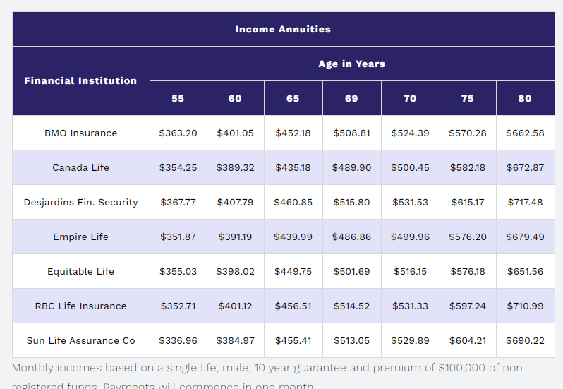
Source: CANNEX quotes obtained on Jan 4th 2021.
Before we define an annuities, a short primer on mortality risk. The idea is not to make you actuaries: we will skip a lot of the technicalities to stay focused on our objective. Denote by \(q(t)\) the fraction of individuals with exact age t who die in that year. The probability that someone born survives to age t is therefore given by
The probability someone of age t survives to age \(t'\) is :
The remaining life expectancy of someone exactly age \(t\) is given by
where \(T\) is some maximal age (where \(q(T)=1\)).
A common form for mortality probabilities that fits the data well, in particular for retirees, is
This is the Gompertz law of mortality. It is easy to estimate Gompertz parameters from data on mortality risk using linear regression of log mortality rates on age (since the equation above is linear). Actuaries estimate these parameters from the pool of individuals purchasing a financial product. Demographers estimate them from the general population. These can yield different estimates, in particular if there is adverse selection (those with lower mortality buy annuities). As economists, we use those parameters as an input to study various household finance choices, including annuities.
A common source of mortality data is the Human Mortality Database (HMD). Lots of what we need to study mortality is available and for many countries. You can create an account for free. Demographers define the collection of cross-sectional mortality rates along with other statistics as a period life-table. People of different ages in a given year make up the life-table. Other life-tables exist, for example cohort life-table, which follow one cohort over time. These can be different when mortality rates change over time or across cohorts. For our purposes, we will use period life-tables. You can upload directly these files into Google Colab. A simple example of a manipulation of a life table is given in the following notebook.
![]()
You will also need the following data file from HMD which you should put in your google drive. We cleaned the raw file a bit for easy loading…
The second component to evaluate an annuity is the discount rate. Annuities are offered mostly by insurance companies. The payouts have default risk, albeit small, and using riskless discount rates probability overestimates the value of annuity payouts. A good measure of the riskiness of insurers is the return on corporate bonds. Denote by \(r\) this discount rate. Complicated models with yield curves or stochastic rates are sometimes used. Since this is not a class in asset pricing, we will use a simple constant discount rate \(r\).
Let us consider an insurer who is willing to cover an individual who has mortality risk described by the series \(q(t')\) for \(t'=t,...,T\). The net present value of a one dollar annuity starting today is given by:
The NPV of a \(A\) dollar annual annuity is simply \(P(t)A\). \(P(t)\) is often called the actuarially fair price of the annuity for a given mortality risk and discount (financial risk).
If one wants to know how much of an annuity can someone buy with \(W\), one can deduce that \(A = \frac{W}{P(t)}\) is the benefit that one can afford for a given wealth. These are the amounts shown in introduction from CANNEX. Given the pricing function, we see that the lower is the interest rate, the less benefit a given amount of wealth an annuity will buy. An annuity becomes more expensive when interest rates are low (just like a bond). Women get less benefit for a given amount of wealth because they live longer (the price is higher). Changes in mortality, drug discovery and medical innovation, are risks that the insurer must take into account. These are hard to diversify. Some of this is done by offering life insurance (hedging) and other is done by re-insurance and derivatives.
The annuity yield is simply the ratio of what it pays out to its price. Hence,
It is also possible to compute yields from internal rate of return calculations. Compare the pricing function of an annuity to the return from holding a bond with the same coupon rate \(r\) and maturity \(T-t\) (omitting the termination value):
Of course, the other difference is that the bond is repaid at maturity while the annuity is not, i.e. the capital is not returned to the client. As we will see later, this will not matter when the consumer does not derive utility from money when dead. But it will matter in other circumstances.
It is easy to see that the price of the annuity is lower than that of the bond. This is intuitive: the bond pays no matter whether the individual is alive or not. The annuity only pays when alive.
An important question is whether annuities found in the market are priced correctly. The money’s worth of an annuity is a useful metric to answer this question. It is the ratio of the fair price \(P(t)\) to the observed price \(\hat P(t)\),
A money’s worth above one indicates the price is more than fair (a bargain) while a money’s worth that less than one indicates an unfair price (fair and unfair from an actuarial point of view, not in terms of inequality, etc). The load, or profit, on an annuity is given by
Load can occur because of administrative costs, risk premiums or even from the possibility that there is adverse selection in the annuity market. A well-known study by Mitchell and co-authors (1999) discusses in great detail money’s worth calculations for annuities in the U.S. Milevsky and Shao (2010) report on the money’s worth of annuities at age 65 for men and women in Canada.
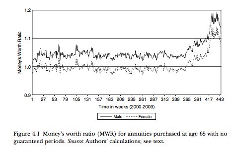
Source:Milevsky and Shao (2010)
Some annuities are sold with a minimum payment guarantee: their payment is guaranteed for a number of years no matter whether someone dies or not. This defeats a bit the purpose of an annuity but avoids “hit-by-the-bus” concerns. Some people might be concerned that they die very shortly after purchasing the annuity. Other annuities are sold jointly on a couple’s lives. Deferred annuities are annuities which start only in the future. One can see the decision to delay claiming public pensions as a form of deferred annuity purchase. Finally, some annuities have an inflation protection (they provide a constant benefit in real terms). Most public pensions are of that sort. Of course, the price of a real annuity is higher than that of a nominal annuity since the insurer must price the additional risk.
The Annuity Market in Canada
Before we describe the private annuity market, it is important to note that the government of Canada already provides annuities. In addition to first-pillar basic income from the Old Age Pension Program, Canada has set up a mandatory public pension system which provides annuity income, proportional to some measure of career earnings, the Canada and Quebec Pension Plan. Together they provide high replacement rates to low earners and lower ones to higher earners. Some workers have also contributed to defined benefit employer pensions which provide them with yet another source of annuity income. These pension plans have come under attack and they are slowly losing ground, except perhaps in the public sector. The bottom line is that a significant fraction of our lifetime income is already converted into annuity income in retirement. Mandatory annuitization is already part of the retirement income system.
On top of this, there is a market for private annuities. The most prevalent forms are variable annuities which are not really annuities but instead an investment product with little to none longevity risk guarantee. The fixed immediate annuity market which will be the focus on is quite small. For example, Milevsky (2013) reports that less 4% of sales are immediate annuities of the type discussed here in the U.S.
For those interested in the annuity market, this report from Moshe Milevsky (2013) is a very exhaustive source of information, including a discussion of where annuities come from…
Who buys annuities?
Data is scant on who receives annuity income outside of public and employer pensions. For this reason, the Retirement and Savings Institute at HEC has conducted a survey aimed at understanding who receives income from a private annuity. Furthermore, this survey asks a number of questions which will be handy latter. Details on the survey can be found here. A clean version of the dataset is available here while the questionnaire here.
Among those 55 to 75 in that survey, 13.4% of Canadians receive income from private annuities. Those who are older are more likely to receive annuities. There is some relationship with income and assets, but that relationship is not as sharp as one would think. Somehow annuity take-up is larger in Quebec. You can read this dataset using the following Notebook and investigate the data. You will need to adjust paths for data files.
![]()
The survey contains questions on knowledge of annuities and how they were bought. The data suggest that knowledge is limited and that most people who purchase an annuity were offered one. This is suggestive of the role of supply in the take-up of an annuity. There are also questions on the reasons behind the decision to buy or not annuities.
Theory
Our objective is to investigate how one should think of annuities as an economist. Consider a setting with two periods, \(t=1,2\). In period 1, the agent can consume \(c_1\), buy bonds, \(B\), or buy annuities \(A\). Each dollar of bonds yield \(r_B\) for consumption in period 2 \(c_2\). For annuities, the fair return of an annuity is \(r_A = r_B/(1-q)\) where \(q\) is the probability of dying before reaching period 2. Hence, each dollar of annuity yields \(r_A\) for 2nd period consumption. An important point to note is that for \(q>0\), \(r_A>r_B\). The return on the annuity (annuity yield) is larger than the return on the bond.
Consider a general utility function \(U(c_1,c_2)\) concave in both arguments. Utility when dead is normalized to zero. We will come back to this important assumption later.
The choice problem is
subject to the short-selling constraint that \(B\ge 0\). Inspection of the problem shows that one can reduce bond holdings by 1 unit and increase annuities by 1 unit without affecting utility from first period consumption. But the result of this reshuffling increases consumption in period 2 since \(r_A>r_B\). Therefore, no matter what is the utility function when alive, the optimal solution is to set \(B^*=0\). The amount of \(A^*\) depends on the consumption plan. But all savings, once consumption has been determined, should be put in annuities. To see this, we can rewrite the problem as
where \(W'\) is savings and \(\phi\) is the fraction of savings held in annuities. Setting \(\phi=1\) is optimal if annuities provide higher returns than bonds (first period consumption unchanged, second period maximized if \(r_A>r_B\)). This result is called full-annuitization. Note that if the load on annuities is such that the return on annuities is lower than bonds, then we get no annuitization.
This is a strong result. It does not depend on using expected utility as long as the consumer has positive marginal utility from consumption in period 1 and 2. The result was first shown by Yaari (1965) but generalized in these terms in Brown, Diamond and Davidoff (2005).
To understand the value of the annuity to the consumer, first write indirect utility for a given \(\phi\) as
Then define the lump-sum that would be equivalent to the annuity as
We can interpret \(LS(W)\) as the bond endowment we must give the consumer to be as well of as he is with full annuitization. It is the minimum asking lump-sum payment he will require for selling the annuity. In standard econ jargon, it is a willingness to accept. Consider the discounted expected utility formulation
One can derive an approximation to the lump-sum. Instead of getting lost in the math, we constructed the following notebook which computes the lump-sum measure and shows that the lump-sum is larger than the net present value of the financial gain from holding the annuity. This is because there are two components to the value of the annuity: an investment component and an insurance/consumption component. The value to the consumer of the annuity is larger than the investment component as the consumer is able to re-optimize his consumption allocation because of the presence of the annuity. For example, he can use the higher lifetime wealth to consume earlier in the life-cycle because he needs to worry less about the risk of surviving to an old age. This can be interpreted as an insurance motive. Turns out this second component is very important in standard calibrations, like the one in the notebook.
![]()
One key extension of this standard framework yields partial annuitization.
Bequests
Consider now relaxing the assumption that the agent does not care about what he leaves behind once he dies. Consider the discounted expected utility setting:
where \(\delta\) is the subjective discount factor.
If he dies, we now consider the utility value (warm glow) of leaving behind whatever he has in terms of bonds to his heirs. Note that there is nothing to pass on with the annuity. The parameter \(\eta\) governs this bequest motive. If zero, we fall back to the model above and full-annuitization under fair pricing occurs. Intuitively, we see that with a bequest motive annuitization implies a trade-off: higher return and consumption value, but one leaves nothing to heirs.
Instead of going through the tedious math and assume functional forms, we will do this in Python… Checkout the notebook above which shows what we get when \(\eta\) is non-zero. Partial annuitization occurs. Remember that given that public programs already provide annuity income, it is possible that private demand for an annuity is zero once bequests are introduced. Hence, this is a serious candidate for explaining lack of annuitization. Lockwood (2012) shows that plausible parametrization of bequest motives can lead to no annuitization.
Limits of the Standard Model
Other extensions may yield partial annuitization, including illiquidity or the presence of residual risk and unfair pricing, taxation and means-testing of other government benefits. There is a large literature which we won’t cover here which focuses on these extensions of the classical model.
Endowment Effects and Cognitive Constraints
Consumers need to part with a fraction of their wealth is they purchase an annuity. A well-known behavioral regularity is that individuals have a higher asking price for something they have already than the bid price to acquire the object Kahneman, Ketsch and Thaler, 1990. This is explained by the endowment effect. In the standard setting, endowment effects are not present and bid and asking price should be close to each other. If \(\phi_0<\phi_1\), where the difference is relatively small,
and
yield \(WTP \approx WTA\). You can check that in the notebook. For a small change in annuitization, both are close to each other.
In practice, if \(\phi_0\) denotes the status quo in the first setting and \(\phi_1\) is the second setting, then \(WTA > WTP\) occurs often in experiments. The consumer is asking a lot more for something he already has than he is willing to pay to acquire it. If endowment effects are present, it is possible that consumers find it difficult to part with some of their financial wealth to purchase an annuity.
It is also possible that consumers have a hard time evaluating an annuity. While the investment value of an annuity is relatively easier to understand, provided valuation is well understood, the consumption value is much harder to grasp. Brown, Kapteyn, Luttmer and Mitchell (2017) investigate the valuation of annuities and in particular relate this to cognition.
They construct an experiment asking respondents for the lump-sum payment they would accept or pay in various annuity configurations centered around what they expect to receive from Social Security (public pensions in the U.S.). The design is constructed around four different frames:
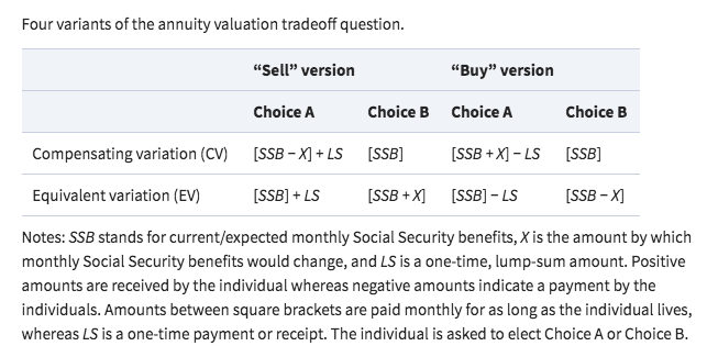
Source: Brown, Kapteyn, Luttmer and Mitchell (2017)
From these frames, CV measures have the potential of being subject to endowment effects since the status quo (Choice B) is present in both. One would expect Buy valuations to be lower than Sell valuations if endowment effects are present. But endowment effects should not be present in the EV valuations since there is no status quo. Hence, a difference between buy and sell lump-sums in the EV scenarios cannot be explained by endowment effects.
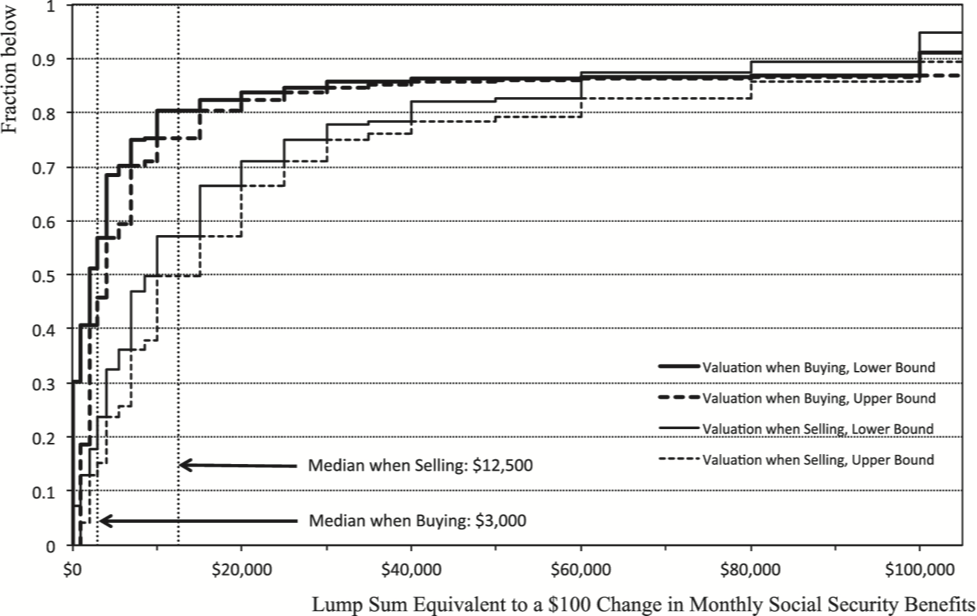
Below are both CV-sell and CV-buy distributions. We find the standard result that WTA (sell) is (much) larger than WTP (buy). The median of both buy and sell is well below the actuarial value. Hence, below the standard value of an annuity in a discounted expected utility model (with no bequest). In particular, the median WTP is quite low (3 000$). These results can be rationalized by an endowment effect model.
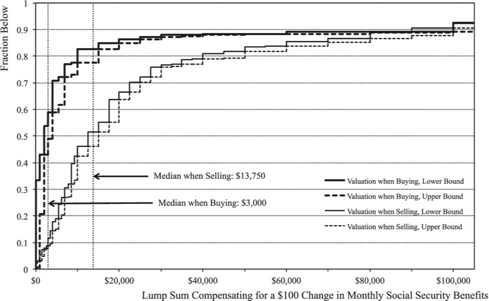
Source: Brown, Kapteyn, Luttmer and Mitchell (2017)
Consider now the distributions for EV in which there is no status quo:
Source: Brown, Kapteyn, Luttmer and Mitchell (2017)
The results are very similar to the CV frames. Hence, we cannot rationalize the discrepancy between the buy and sell valuations by endowment effects. A hint that respondents are having trouble is that there is a negative correlation between CV-sell and EV-sell when in fact, these are essentially the same trade-offs.
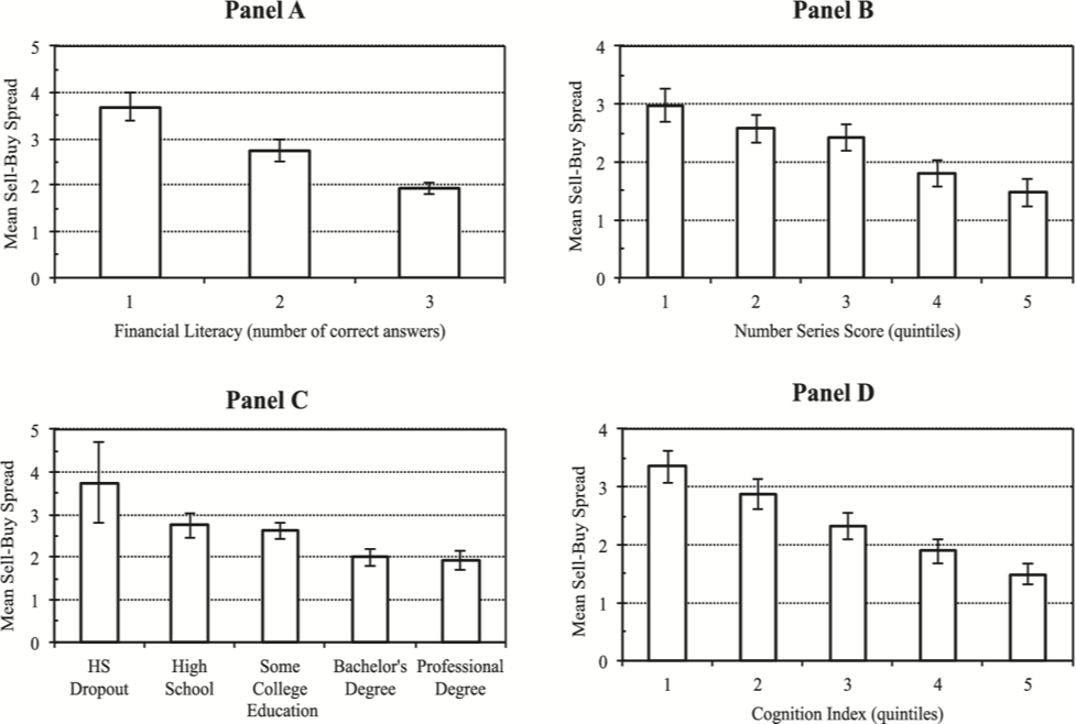
Instead the authors conjecture that when people have a hard time valuing a product, there will have a reluctance to trade, which means high reservation price to sell and low willingness to pay. If this is correct, then the spread should correlate with known correlates of cognition and financial knowledge. They use the difference between (log) CV-Sell and CV-Buy as a measure of the spread. The larger is that indicator, the larger the unwillingness to trade. For more than 80% of the sample, this difference is positive.
The next figure from the paper shows that there is a clear negative relationship between the average spread and various measures.
Source: Brown, Kapteyn, Luttmer and Mitchell (2017)
The relationship with education is in line with the conjecture but can also mean a number of things. But consider the other measures.
First, there is a cognition index. Cognitive abilities steam from two forms of intelligence, fluid and crystallized. Fluid intelligence allows us to perform new operations, computations and solve new problems. Crystalized intelligence is about mostly experience. While Crystalized intelligence tends to plateau at some point in the life-cycle, our fluid intelligence decline starting in our twenties. Taken together, this implies that our cognitive abilities to make financial decisions is likely to follow an inverted-U with age and decline eventually. Agarwal et al. (2009) have this picture showing the relationship.
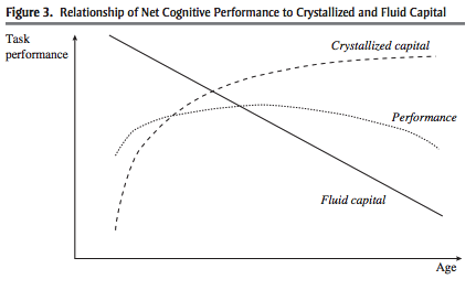
Source: Agarwal et al. (2009)
This means that for annuity purchases, which occur late in life, there could be a role of cognitive abilities in explaining the difficulty in valuing annuities. Brown et al. (2017) use a cognitive index score which aggregates three different measures. They find a negative relationship with the buy and sell spread which is consistent with their conjecture.
A second measure Brown et al. use is a measure of numeracy, the Number series score. Now someone can be good at solving problems, have high fluid intelligence, just not one that helps with problems involving math or numbers. It is hard to argue that Math is not useful to value annuities. Hence, they use a numeracy measure which counts the success of respondents at filling math sequences. They find a negative relationship with buy and sell spreads, again consistent with the conjecture.
The third measure is financial literacy, which measures something distinct from cognitive abilities and numeracy. One could have very good cognitive abilities, be good at Math, yet have trouble with financial concepts such as compounding, inflation and diversification. Lusardi and Mitchell in a series of papers have proposed three questions on these topics (see Lusardi and Mitchell (2014) for a survey). Brown et al. (2007) simply count the number of correct answers. Again, a negative relationship between spreads and financial literacy.
The takeaway is that valuing annuities is hard and that this difficulty is related to cognitive abilities, financial literacy and numeracy. This yields a number of hints of how to increase annuity take-up, if that is optimal from a discounted expected utility point of view.
Interventions
There is a flourishing literature on interventions to increase annuity take-up. Here we cover a few studies.
Framing of Investment vs. Consumption Value
We saw earlier that the value to consumers of an annuity is composed of an investment and consumption-insurance value. What if consumers have trouble considering the value jointly. If consumers solely focus on the investment value (how investing in annuities impacts returns), they may underestimate the total value of buying an annuity. Furthermore, the annuity may appear riskier than the bond since it only pays when someone is alive. Brown, Kling, Mullainathan and Wrobel (2008) present respondents with several vignettes in two different frames. Here is the example of Mr. Red.:
Consider the investment frame:
Mr. Red invests $100,000 in an account which earns $650 each month for as long as he lives. He can only withdraw the earnings he receives, not the invested money. When he dies, the earnings will stop and his investment will be worth nothing.
Now consider the consumption frame:
Mr. Red can spend $650 each month for as long as he lives in addition to social security. When he dies, there will be no more payments.
Mr. Red is pitted against another vignette of someone who did not have an immediate life annuity. When Mr. Red is put against someone with a traditional savings account, 21% think Mr. Red did well when using the investment frame and 72% when using a consumption frame. Hence, the nature of the frame is very important to annuity choices.
Framing and Complexity
Brown, Kapteyn, Luttmer, Mitchell and Samek (2019) conduct an experiment using again the sell-buy spread but this time looking at whether i) complexity reduces demand, ii) whether inducing people to think about how to spend down assets increases demand. One can think of point i) as being directly related to the results of their previous study where they showed that difficulty in valuing annuities was associated with cognitive abilities, numeracy and financial literacy. Complexity is added in terms of mortality risk (which increases the computational burden) and in terms of information about qualification which is unnecessary to the valuation task but needs to be discarded by respondents (adds complexity). The other treatment is aimed at avoiding narrow framing, where respondents focus on the investment task, forgetting about the consumption or insurance value of annuities. They do this by simulating an interaction between the vignette person and a financial advisor who explains the risks one runs by choosing how to spend down saving. Table 3 of the paper shows that complexity increases the buy-sell spread by 13%, hence diminishes valuation quality, while the second framing, aimed at eliminating narrow framing, decreases the buy-sell spread by 14%, mostly by increasing the Buy willingness to pay.
Product Design
There appears to be some demand for increasing annuities or flexibility. For example, Beshears et al. (2014) show that there is an increased demand for annuities when some flexibility is introduced, for example the possibility of having an escalating annuity rather than flat, or the possibility to withdraw some portion without penalty. Of course, flexibility comes at a cost in terms of complexity which we have shown tends to lower demand for annuities.