Savings

Facts
Stocks and Flows
Over the life-cycle, people earn income from work but also from pensions and other sources. They use this income to spend on goods. They sometimes also decide to leave some to their heirs as bequests. The basic point is that there is no need for a one-to-one relationship between when we earn income and when we spend it. Luckily, we can save some income for later, for example when we earn a lot and we can borrow, for example when income is low. In practice, we observe large flows of saving, and then dissaving over the life-cycle. Some of these flows are mandatory, i.e. consumers are forced to make them. For example, paying mandatory pension contributions reduces potential expenditures today against a promise to receive pension income in the future. This allows to spend on goods and services when old. Paying taxes also involves saving since lots of government spending is devoted to the young (who earn no income) and the old, who for example consume more health care. These intergenerational transfers involve saving and borrowing. In this set of lectures, we will be mostly concerned with voluntary private savings which occurs on top of all the life-cycle and intergenerational transfers that occur. Because savings can be measured as stocks and flows, it will be useful to think of financial wealth as a stock (accumulated savings), with active savings (contributions and withdrawals) and passive savings (returns and capital gains or loss) being the flows. Let the stock of all savings, financial wealth evaluated at market value, be \(w_t\). Denote by \(s_t\) the contributions (when positive) and withdrawals (when negatives), \(r_t\) the effective rate of return. The component \(r_t w_t\) is unrealized capital gains and returns. Financial wealth evolves according to
Even if \(s_t=0\), financial wealth may go up because of capital gains and interest. Alternatively, it is possible that \(w_{t+1}=w_{t}\) even if \(s_t \neq 0\). Hence, reconstructing stocks from flows and infering flows from stocks requires good data on the various flows. Turns out we have limited information on financial wealth, stocks, but also on flows, savings and dissavings. Administrative data in most countries, with the exception of some scandinavian countries, is not available on savings stock and flows such that we could reconstruct the equation above from data. One of the reasons is that governments do not generally tax stocks, hence do not collect data on them. Hence, we must resort to surveys to get most of our information on savings flows and stocks.
Canada has a cross-sectional data infrastructure that allows to get a picture, once in a while, of how much people save (or have accumulated). Statistics Canada runs two surveys, each with their specific purpose, that allow us to paint some portrait of private savings: the Survey of Household Spending and the Survey of Financial Security (SFS) . The Survey of Household Spending gives us information on income, spending and some measures of direct active savings and dissavings. This is a decent survey for flows. For stocks, the Survey of Financial Security (SFS) allows us to construct the balance sheet of Canadians. The SHS is run annually while the SFS is run every five years or so (1999, 2005, 2012, 2016). For researchers at Canadian universities, public micro-use files (PUMFS) can be downloaded from ODESI.
Take flows first. Measuring saving contributions can be done in a number of ways, each imperfect. Sometimes, respondents are asked directly whether they have contributed to a savings account. This gives direct measurement of \(s_t\), active savings. But it is something hard for people to remember the net savings they make across different saving vehicles. Simply looking at their end and starting balance does not identify active savings. Sometimes, they are asked instead information on spending, \(c_t\) and income \(y_t\) and an implied savings variable can be created \(s_t = y_t - c_t\). But this measure involves a few difficulties if we are to use the term active savings, including how to deal with durable spending and income from dividends and interest which may have been included in the definition of income, but left in the account (not realized). Taxes are not always easy to deal with either. Knowledge of active savings is not enough to reconstruct the wealth equation since the return component is only partially accounted for. There is also the question of how to include pension contributions and taxes in this definition when only gross income has been reported. Finally, an alternative is to construct savings by asking for changes in wealth at two points \(s_t = w_{t} - w_{t-1}\). This is not a direct measure of \(s_t\) as defined in the equation above since it will include unrealized capital gains, \(r_t w_t\).
The next figure from SHS shows average consumption and spending at the household level by age in 2009. The information is aggregated by age groups. Income is hump-shaped. We see that spending is also hump-shaped. But we see that savings occurs mostly in the middle of the life-cycle. Interestingly, we do not observe dissaving at older ages. One important point to make is that a period age-profile does not necessarily represent how a cohort behaves over the life-cycle. In other words, the 65 year olds are from a different generation than the 25 year olds in the plot. If there are large differences in income or other characteristics across cohorts, the period profile is a poor guide to what happens to a cohort over the life-cycle. When repeated cross-sectional data is available, one can use a synthetic cohort method. Attanasio (1998) is a good example applied to savings.
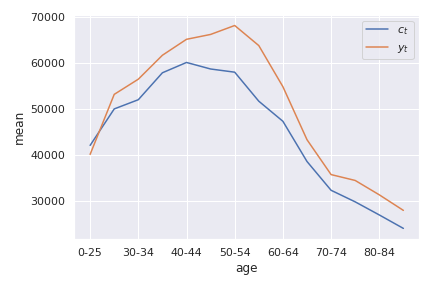
Source: Calculations from Survey of Household Spending, 2009
You can check how these data manipulations are done directly in Google collab once you have downloaded the PUMFS to your google drive.
![]()
We can compare the two definitions of savings rates across income quintiles. The next figure shows the average savings rate using the consumption definition and using the first difference in wealth. While the pattern is similar and slopes are similar, there are some differences between the two measures. Interestingly, those with higher income save more as a fraction of income than those with lower income. This has a number of implications for wealth inequality.
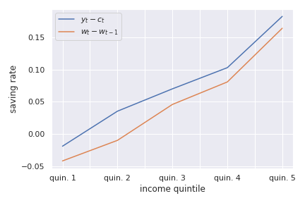
Source: Calculations from the Survey of Household Spending, 2009
Private savings can take many forms. Individuals save using a multitude of products. The first useful distinction is between registered and unregistered funds, at least in Canada. We refer to savings as either being registered or unregistered, depending on whether they are subject to specific tax treatment or not. Unregistered savings essentially takes the form of cash and deposit accounts, bonds and stocks that are held outside of tax-preferred saving vehicles. Registered forms of savings include Tax-free Savings Accounts (TFSA) and Registered Retirement Savings Plan (RRSP). Since unregistered savings are made out of money that has been taxed, we say that saving contributions are taxed. Unregistered savings are also taxed through the taxation of returns (dividends, interest income). But they are not taxed on the stock or amount owned (there is no wealth tax in Canada), nor are they taxed when we take money out of our accounts, except for the partial taxation of capital gains. We say that they have a TTE tax treatment, for contribution (T), returns (T) and withdrawals (E). TFSAs are TEE while RRSP are EET. There is one less T, the middle T compared to unregistered funds. In the next figure we plot the fraction of respondents in SHS who contribute and withdraw funds from RRSPs. We see that RRSP contributions are hump-shaped while withdrawals increase around the time of retirement. But there are withdrawals before retirement as well. TFSAs are more recent (introduced in 2009) and therefore were not in place in 2009 when this data was collected.
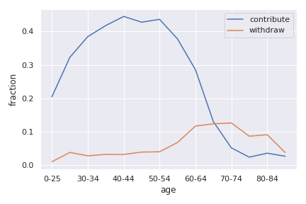
Source: Calculations from the Survey of Household Spending, 2009
Contribution rates and amounts (conditional on contributing) are quite skewed in terms of income as the next figure shows.
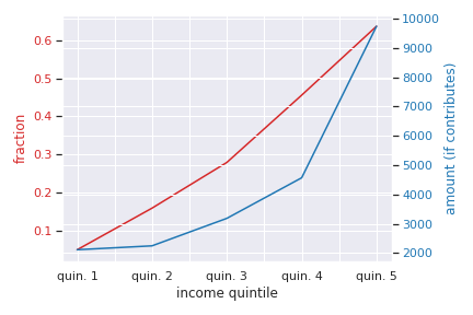
Source: Calculations from the Survey of Household Spending, 2009
Registered savings are very popular. For example, Statistics Canada reports for 2018, a total of 43.5 billion dollars in RRSP contributions while the number of 66 billion for TFSA in the same year.
Adding unregistered to registered savings, we get liquid wealth or financial wealth (\(w_t\) for our purposes). Implicitly, this allows to make the distinction with another form of wealth, the stock of real assets, such as cars and real estate. The Survey of Financial Security allows us to draw a good portrait of financial wealth. In the next figure, we zoom-in on the near retirees (age 55-65). We first look at the composition of financial wealth by education, a good marker of lifetime income.
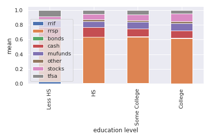
Source: Calculations from the Survey of Financial Security, 2009
We see that nearly half of financial wealth is in RRSPs and that this share is roughly similar across education groups. The share of cash, or bank accounts is smaller for those with higher education and the fraction in stocks slightly increasing in education (also mutual funds). The next figure shows the distribution of financial wealth as a fraction of after-tax income.
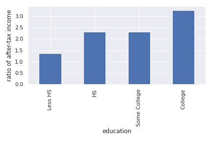
Source: Calculations from the Survey of Financial Security, 2009
We see that financial wealth is larger relative to income for those with higher education. We could say that they save more, but from the wealth equation above, we understand that this is not necessarily true. They could have saved less but obtained better returns from investing. On average, college-educated households have 3 times their after-tax income in financial wealth compared to roughly 1.25 for those with less than high school. In fact, averages mask a lot of heterogeneity and considerable skewness in the distribution of financial wealth. The next figure shows an histogram of the distribution of financial wealth relative to after-tax income. We see that more than 25% of respondents have close to no financial wealth. While income is roughly log normal, wealth is typically much more skewed. Outliers can impact estimates, particularly when using survey data. Using medians and other statistics less sensitive to outliers can be useful.
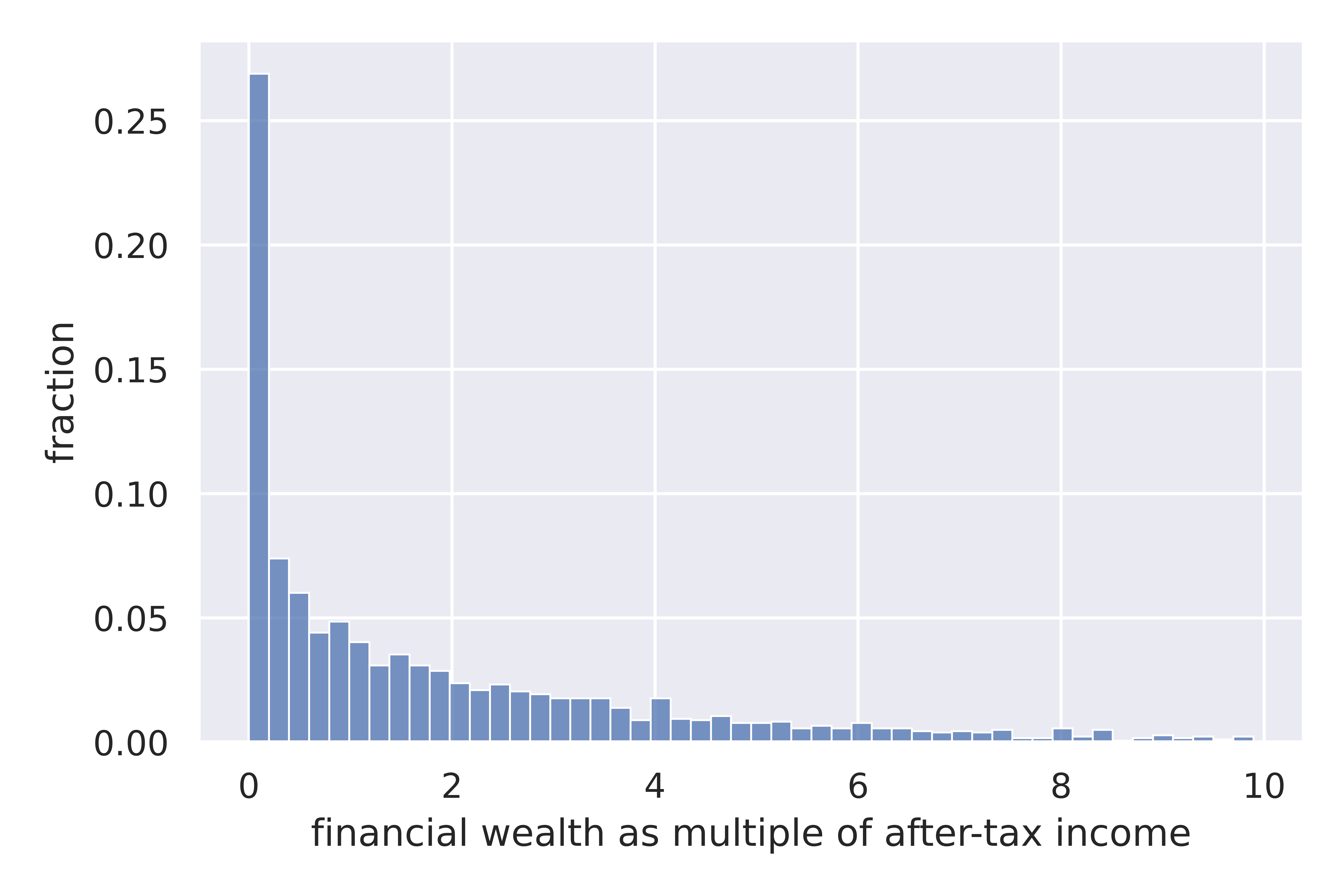
Source: Calculations from the Survey of Financial Security, 2009
These calculations using the SFS can be replicated using this notebook.
![]()
Replacement Rates
Later, we will ask the question of whether or not people are savings enough for retirement. Before one even contemplates to make the decision of how much to save, it is useful to ask what the public pension system, and employers, already replace in terms of lifetime income for retirement. Retirement income systems are complicated and messy. A good overview of the system is available here. But to summarize it succinctly for our purposes:
First pillar: Old age security (OAS) and guaranteed income supplement (GIS). They are not based on career earnings, but provide a flat pension which is clawed back at different rates depending on other retirement income.
Second pillar: Canada (and Quebec) Pension Plan provide a benefit which is a function of lifetime earnings against contributions which are made while working.
Third pillar: Employer Defined benefit and Defined Contribution plans. DB plans provide an annuity against contributions made while working. Define contribution plans set an accumulation scheme for workers to contribute, sometimes with employers matching their contributions. They have access to accumulated funds upon retirement.
Fourth pillar: Private retirement savings
The top three pillars interact with each other in complex ways. In addition, the tax system impacts disposable income, while working and when retired. To compare to the system in other countries, the OECD Pension at a Glance publications are very useful.
One common measure of the generosity of a retirement system is the ratio of disposable income after retirement to that before retirement, an effective replacement rate. Both measures of pre and post-disposable retirement income can be computed a number of ways, sometimes after tax and sometimes before tax. Sometimes average career earnings are used while other times earnings at some age are used. When defined contribution plans are in play, one needs to decide how to annuitize their value to compute an annual flow of disposable income. A similar problem arises with other stock variables.
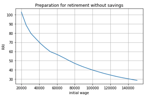
To showcase the effective replacement rates in the Canadian retirement system, we use a retirement income simulator produced by the Retirement and Savings Institute at HEC, the CPR. That calculator allows to project someone’s outcomes all the way to retirement based on inputs regarding earnings and other characteristics. It can also be used on a dataset of potential cases. Here, we show an example which computes the Retirement Readiness Index, the ratio of consumption in retirement to consumption at some age when working, for various levels of labor earnings. Retirement income includes only public pensions in this example (first and second pillar). We see that the net after tax replacement rate is close to 100% at low levels of earnings but quickly drops. For someone earning more than 120 000$ per year at age 35, the replacement rate is expected to be lower than 20%. Hence, the Canadian RIS is one where 3rd and 4th pillar savings is important. Turns out the third pillar is weaker than it was, both in terms of coverage but also in terms of plans offered. DB plans are slowly fading away in favor of DC plans, which leave the saving decision to the worker. Finally, recent developments have seen the introduction of an hybrid type of plan, target date plans.
You can use the CPR directly in a Google Collab Notebook. Here is the link.
![]()
Theory
The Life-cycle Benchmark
How much should people save?
It is useful to first look at a benchmark. A natural starting point is the life-cycle model. The life-cycle model has a long tradition in economics and finance. A good summary is given in Browning and Crossley (2001). In what follows, we will use a three-period model, \(t=1,2,3\). Why three? It will become clear later on. The first two periods are periods where the individual works and earns labor income \(y_t\), net of taxes and pension contributions. Otherwise, denote \(\overline{y}=\frac{y_1+y_2}{2}\) to be average career earnings. For most of the analysis, we will focus on the case where \(y_t = y\) for \(t=1,2\), hence \(\overline{y} = y\). The last period is one where he is retired. He gets in that period income from pensions, denoted \(\phi \overline{y}\), where \(\phi\) is a replacement rate. You can think of this rate as the RRI from the CPR calculator we used above. We will abstract from uncertainty for now. For simplicity assume the individual has no wealth start with. He can save with a rate of return \(r\) which is also the rate at which he can borrow.
Consider preferences of this consumer. A natural starting point is to consider discounted utility from the consumption plan \((c_1,c_2,c_3)\). If you are not familiar with discounted utility (DU), you can look at this lecture from my intermediate micro class. Discounted utility is given by
The budget constraint is such that the present value of consumption should not be larger than the present value of income:
where \(R = 1+r\). Hence, saving and borrowing is allowed.
The first order conditions from this problem yield three equations:
Consider a very simple form of the utility function (iso-elastic):
This leaves us with an equation determining the path of the optimal consumption plan
Denote \(\eta = (R\delta)^{\rho}\) to be the desired growth factor of consumption. If \(\eta>1\), for example because the consumer is very patient, consumption is initially lower and then higher in the last period. If \(\eta<1\), for example because the consumer is very impatient, the consumption plan is lower in retirement. The parameter \(\rho\) controls the slope of this consumption plan. For example, we can interpret this parameter as:
using the fact that \(\log R \approx r\) for small \(r\). The consumer is willing to substitute consumption now for retirement when the interest changes if he has a high value of this parameter. Hence, we call this parameter the Intertemporal elasticity of substitution (IES). A consumer with a high IES may want to save, simply because he is facing a rate of return that is high and/or he is very patient. We can call this the investment motive to savings. It is a function of both the interest rate as well as preferences. We reduce the first order conditions to obtain
and finally, using the budget constraint to pin the level of consumption, with \(PV_{y}\) the RHS of this equation (present value of income):
And using the Euler equation for other periods, we get:
A number of remarks are in order. First, consumption does not necessarily follow the path of income. We see that the consumer wants to consume part of the present value of income \(PV_{y}\). But this is orthogonal (unrelated) to the path of \(y_t\). If his income is high relative to other periods, he is likely to save while if his income is low, he is likely to consume out of savings. To see this, consider for example first period savings, if \(y_1 = y_2 = y\) and \(\eta = 1\). We get
Provided \(\phi<1\), the consumer saves part of his first period income. He will also do the same in period 2. He has a life-cycle motive to save, because his retirement income is lower than his income when working. The marginal utility of consumption in retirement is larger than when working if he does not save. Hence, he can increase discounted utility if he saves from his first and second period income.
The case with \(\phi \neq 1\) is not different but will involve the combination of a life-cycle motive and investment motive to save.
A third key motive to save is the precautionary motive. To see this motive, one needs to introduce uncertainty. Consider the possibility that second period income can be \(\underline{y}_{2}\) with probability \(p\) and \(\overline{y}_{2}\) with probability \((1-p)\) with \(y_2 = p \underline{y}_2 + (1-p)\overline{y}_2\). Uncertainty induces a mean-preserving spread in income in the second period. Given the concavity of utility it means that marginal utility is high when income is low and vice-versa when income is high. The first order condition, using discounted expected utility, for the trade-off between 1st and 2nd period consumption is now given by
where the \(E\) operator is with respect to the income shock. If we evaluate this first order condition at the optimal plan without uncertainty, we see that we will change the optimal consumption plan if the RHS is not the same. If the marginal utility of consumption is linear in consumption, there is no change in the optimal consumption plan (since uncertainty induced a mean-preserving spread). This is for example true when utility is quadratic. But for other cases, it will generally not be the same. In particular, for the case of the iso-elastic utility function above, the right-hand side will be larger, because the marginal utility is convex (the third derivative of utility is positive, what we call prudence). Hence, due to Jensen’s inequality \(E u'(c_2) > u'(E c_2)\). If this is the case, then the consumer must increase the LHS of the equation, which implies reducing first period consumption and therefore increasing savings. This is the precautionary saving motive. The consumer wants to build a rainy day fund to face the possibility of getting low income in the second period. He wants to do this because he is averse to downside risk. This goes beyond risk aversion. While this is not something we will study in what follows, there is a large literature on this saving mechanism. Lusardi (1998) is a good entry point in the literature for a test. For the theoretical underpinning of the precautionary motive and prudence, see Kimball (1990).
Are Consumers Saving Enough for Retirement?
We will focus on the life-cycle motive for what follows. What is the potential for the standard theory to answer whether or not people are saving enough for retirement? There are a number of studies who have looked at this question, in particular for the U.S. Four approaches are taken:
retirement-consumption approach: This early approach tries to test one of the predictions of the model above. If consumers act according to the model above, there should be no jump in consumption at retirement. Consumption is a function of the present value of income and not its path. Since the path of income is mostly known and anticipated, consumption should not drop at retirement.
For example, take the model above and consider the ratio of optimal third period consumption to second period consumption. It yields \(\eta\), and similarly for period 1 to period 2. Hence, there is no jump in consumption.
This produces an implicit test of retirement saving adequacy. The first attempt at exploiting this is prediction is Banks, Blundell and Tanner (1998).
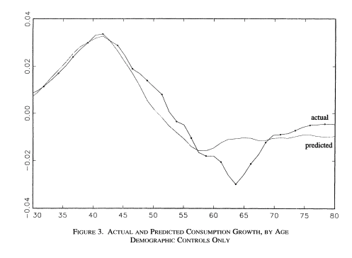
Source: Banks, Blundell and Tanner (1998), Figure 3.
Upon further examination, across a number of countries, the general conclusion is that a large fraction of this is due to work-related expenditures dropping at retirement, substitution to home production, retirement being partly a surprise, when a shock occurs. A simple extension of our three period model would consider the possibility that the marginal utility of consumption in \(u'_3(c_3)\) is lower because more leisure is now consumed and substitutes for consumption. Allowing the age-dependent marginal utilities opens up a world of possibilities in terms of allowing for a consumption drop in retirement which is optimal and does not signal lack of preparation. For empirical tests involving examinations of the source of the drop and exploiting changes in the retirement system see Battistin et al. (2009). Hence, the general conclusion from this approach is that this evidence is unlikely to support widespread lack of retirement preparation.
Accumulation modeling approach: Another approach has been to use observed wealth at retirement and to try and match it to what would be predicted from a fully rational model using detailed life histories of consumers. This backward-looking approach tries to reconstruct wealth from the life histories and the predictions from a life-cycle model. This approach is taken for example by Scholz et al. (2006).
The model above yields a prediction for how much wealth should be accumulated in retirement. The equation for optimal wealth at the beginning of period 3 is messy, but it depends generally on the various variables of the model:
In particular, it will depend on the work income history, the replacement rate, the interest rate and finally preferences. If we divide by \(\overline{y}\), this gives us a measure akin to what is plotted in the figure above in terms of financial wealth as ratio of income. We can compare actual wealth to optimal wealth. This is what Scholz and co-authors do. The key figure in that paper is the following:
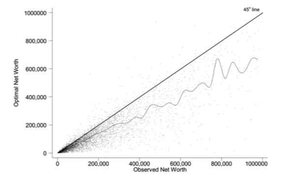
Source: Scholz et al. (2006), Figure 2.
On the Y axis, we have what predicted optimal wealth for respondents in an American Survey with very detailed retrospective information. A complex life-cycle model is used to produce these predictions. On the X axis, we have how much individuals have actually saved. Now, it is perfectly possible for optimal wealth not to be equal to actual wealth. But one would expect a cloud of points on the 45 degree line if this was simply the result of noise. If points are all above the 45 degree line, it would mean that these respondents are saving less than what a model would predict. Turns out, 80% of respondents are below the 45 degree line. This would indicate that they save more than what the model predicts. While some explanations are possible for over-savings, including a bequest motive, this study would suggest that 20% save less than what the model would predict. One attempt to apply this approach to Canada is Liu et al. (2013).
The following notebook takes our three period model and computes optimal wealth.
![]()
Decumulation modeling approach: One could take a different route to the modeling approach by using wealth and expenditures at the time of retirement, using a life-cycle model to determine the path of expenditures in retirement and see if wealth at retirement is sufficient to sustain the path of expenditures. An example is given by Hurd and Rohwedder. They find a result similar to Scholz et al. (2006). This is an approach which shows promise but has been little adopted in the literature.
Replacement rate approach: The standard approach popular in policy circles is actually to compute the RRI in a way similar to what the CPR does and then define a threshold for whether or not the replacement rate (RRI) is sufficient. The difficulty is setting the threshold. As Skinner (2007) explains, models such as those by Scholz et al. (2006) generate explicit thresholds. The particular assumptions about the model, and the heterogeneity across consumers, will impact this threshold. Studies following this approach will use relatively loosely specified thresholds based on observations on expenditures prior and after retirement or consumers. In Canada, examples are given by Wolfson (2011), McKinsey (2014) and quite a recent study by the Retirement Savings Institute (2020). For example, the RSI and McKinsey studies use 80% as a threshold for those in the first income quartile and 60% for others. These studies obtain results which suggest that a targeted group does not meet the threshold. The size of the group varies across studies, from 15% to 50%. This summary from Baldwin (2018) is a good entry point into the Canadian debate.
Overall, a good summary of all this evidence is that a relatively significant group does not appear to be saving enough. What saving enough means varies depending on the actual benchmark one uses, which explains some of the differences across approaches and studies. But an important conclusion is that the lack of retirement is not widespread as some would believe. This is an importance nuance, in particular when discussing policy options to increase retirement preparation.
Why are some not saving enough?
There are many reasons why some may have a hard time saving and planning for retirement. Here we will focus on discounting. Impatience certainly plays a role. After all, the optimal saving formula above does suggest that when \(\delta\) is low, consumers will save less, because of the investment motive. They simply do not find returns attractive relative to their impatience which leads them to neglect the future. What is the evidence on discount rates? Well, it does start early in life…
Harrison, Lau and Williams (2002) is a good example of eliciting discount rates from Denmark using Multiple Price Lists.
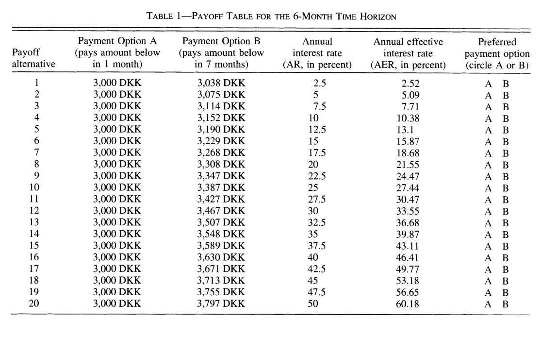
Source: Harrison, Lau and Williams (2002)
with the following relatively high annual discount rates which vary somewhat in the population,
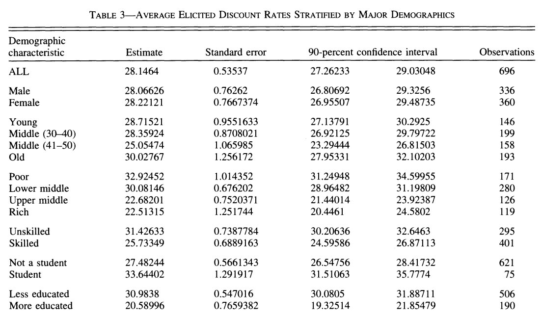
Source: Harrison, Lau and Williams (2002)
But having high discount rates is not sufficient to generate dispersion in retirement savings of the scale we observe. Furthermore, a model would have a hard time explaining why so few workers choose to contribute to voluntary retirement plans, when offered a relatively sizeable match for their contribution by their employer. Turns out, we may want to dig deeper into discounting to understand these behaviors.
Implicit in the EDU (exponential discounted utility) framework is that individuals use a fixed discount rate at different horizons in the future. Over short time periods, the discount function converges to:
where \(\nu\) is the discount rate. Note that \(\nu\) is constant and does not depend on \(t\).
A high discount rate certainly leads to lower savings but will not in general explain why a significant fraction actually holds little to no savings, even when faced with large incentives to save.
Turns out that there is plenty of experimental evidence that we discount the immediate future (short term) at a much higher rate than we discount the future (longer term). For example, a survey of the experimental literature shows that discount factors are highly non-linear in the horizon considered (Frederick, Loewenstein and O’Donohue, 2002).
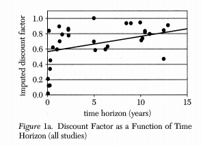
Source: (Frederick, Loewenstein and O’Donohue, 2002)
We see that there is an increasing relationship with the horizon, something that violates the assumption of the standard model. Thaler (1981) presents an intuitive example. Suppose you have to pick between one apple today and two tomorrow vs. picking between one apple in one year and two in a year plus one day. While you may want to pick one apple today vs two tomorrow, you are very unlikely to pick one apple in one year (what’s the difference of a day in one year to get two!). This simple example shows that exponentially constant discounting is unlikely to hold. Thaler calls this the common difference effect (our preference shifts towards the larger outcome when the delay increases).
Turns out that there is even neurological evidence on this relationship. McClure and colleagues (2007) . show in an experiment that the part of our brain which is very sensitive to immediate rewards (\(\beta\) regions) lights up much more strongly when choices have a short horizon than when the horizon is longer. In this last case, activation of regions of the brain associated with planning and deliberation (\(\delta\) regions) is more prominent.
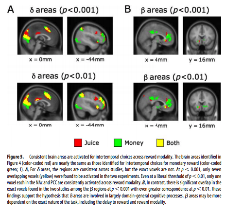
Source: McClure and colleagues (2007)
This is a problem for the life-cycle model to explain saving behavior. It leads to time-inconsistent behavior as first shown by Stotz (1955). The only model which is time consistent in the class of models with sums of utilities is the model with an exponential discount rate. What is time inconsistency? In our context, it implies that it may be optimal in period 1 to plan a certain level of consumption in period 2 but that once we reach period 2, the consumer would like to implement a new plan, despite the fact that nothing has changed. Why is this important? If it is optimal to delay saving to the second period but the consumer decides not to save in period 2, this means that saving for retirement never occurs, despite being optimal from the point of view of the first period… Lots of nice results that we often use to solve these models break when we have time-inconsistent preferences.
The most popular form of the present-bias model was proposed by Laibson (1997). It is often called the \((\beta,\delta)\) model of discounting. Consider our three period model and consider the following modification to the objective function:
Close inspection of this function reveals that the marginal rate of substitution (MRS) between 1st and 2nd period consumption has a \(\frac{1}{\beta \delta}\) term while the trade-off between 2nd and 3rd period consumption has \(\frac{1}{\delta}\). Provided \(\beta<1\), this will tilt consumption towards period 1 relative to the plan with \(beta=1\). We index the objective function with the time at which decisions are made. The consumption plan will be based on these MRS and relative prices from the intertemporal budget constraint. But now consider the moment the consumer reaches period 2. He now maximizes
The MRS now has a term \(\frac{1}{\beta \delta}\). Hence, the valuation of second period consumption is now higher than when the plan was made in the first period (with \(\frac{1}{\delta}\) in the MRS for the trade-off between 2nd and 3rd period). Consumption will be revised upward relative to the original plan. Hence, the total amount of saving is lower when reaching period 3. This is despite the fact that the agent is generally patient over longer horizons.
Experimental evidence suggests that \(\delta\) is close to one while \(\beta\) may be closer to 0.5-0.6. This may lead to large effects on behavior.
This type of mechanism leads to procrastination. When there is a delay between the cost of an action and its benefits, a consumer with present-biased preference will delay actions. Perhaps the greatest example of this type of behavior is smoking cessation. But it also applies potentially to saving since saving means reducing consumption today (the cost) for a delayed reward (interest and consumption) in the future. It also leads to procrastination in terms of actions which imply a fixed cost. For example, workers may need to voluntarily enroll in a savings plan to save for retirement. If there are fixed costs associated with enrolling (filling up paper work, etc), they may always delay the action. Therefore the presence of fixed costs may exacerbate the effect of present-bias preferences on behavior.
If a consumer is smart about present bias, he way take actions to force his future selves to take different actions. Although he will generally not be able to implement the optimal plan, he may avoid the more damaging action of acting in a naive ways. Some models allow agents to be sophisticated or naive, to a different degree, about present bias. A formalization of those ideas is found in O’Donoghue and Rabin (1999).
The following notebook allows to solve a simple present-bias model.
![]()
Interventions
While education and financial literacy could be used to increase saving of those who save too little, we will focus in this lecture on interventions which involve making changes to the choice architecture for savings or mandating savings.
Choice architecture
The main trust of the argument for choice architecture is found in Thaler and Sunstein (2003). No matter what we do, we frame decisions in a certain way. They use the example of defaults. An opt-in choice architecture is one where the default is no action. Most purchase situations are framed in this way. We must take action to purchase a product, enroll in a program. An opt-out choice architecture is one where we are enrolled by default and we must take action to opt-out. Hence, the default is action. None of these are neutral as present biased individuals, if faced with fixed cost, are more likely to stay enrolled in an opt-out and not be enrolled in an opt-in. Hence a choice must be made and they argue that it is perfectly acceptable to nudge consumers when a particular option is more desirable than the other. This principle is called libertarian paternalism. Compared to mandatory choice, It allows those who are nudged into an option they dislike a lot to change their choice. That principle has led to a large host of interventions to nudge consumers.
Automatic Enrollment
One of the most successful choice architecture interventions has been the use of opt-out defaults in private pension plan enrollment. Madrian and Shea (2001) show that when a particular company switched from opt-in to opt-out, enrollment increased substantially. This is often called Automatic enrollment in policy circles. Recently, new evidence is emerging that perhaps automatic enrollment raises savings in the short term but that in the long-term saving outcomes are the same Choukhmane (2019) . Others have looked if consumers driven to save more by automatic enrollment increase debt by not adjusting their spending Beshears and colleagues (forthcoming). We will dig into these studies in class.
Automatic Escalation
While Automatic enrollment tends to increase enrollment, it does so at relatively low contribution rates. Inertia and present-bias lead typically consumers to stay at the default in terms of contribution rates. This can lead to low level of savings. Another intervention, named Save More Tomorrow (SMT) by the authors is designed to increase contribution rates (Thaler and Bernatzi, 2004). To make increasing contribution rates less painful, workers commit to allocating a portion of future salary increases to savings. This exploits both present bias as well as the lower sensitivity of consumers to gains rather than losses. Since salary increases are a gain from the reference point of today, lowering that increase is less painful than lowering salary at the reference point. The intervention is largely successful in raising saving from less than 3.5% of earnings to 13.6%. The authors have been very successful with this idea. In class, we will review critically the evidence.
Mandatory Savings
The classical literature dating back to Feldstein (1974) has documented a crowdout effect of mandatory savings, for example through public pensions. Three good examples are Attanasio and Rohwedder (2003) , Gale (1998) and Messacar (2018). If we mandate people to save, they will reduce their private savings. Hence, it is unclear whether mandating people to save will increase overall retirement savings, and ultimately retirement incomes, if that was our objective. Chetty and colleagues (2014) find that more than 85% of savers in Denmark appear to be passive savers, because of inertia, potentially created by present bias. Hence, they do not adjust savings when mandatory savings change. The other 15% behaves a bit like the standard model would predict, i.e. they reduce savings when mandatory savings change.