Investing
Facts
Intuitively, financial wealth evolves according to
where \(w_{t}\) is wealth \(s_{t}\) is current savings (\(y_t - c_t\)) and \(r_{t}\) is the investment return on wealth. That return could explain lots of the variation in wealth we observe in the data, both because some are able to get better returns on average or they are better able to control variation of those returns and associated consequences. The figure below shows statistics on the return on wealth from administrative data in Norway (Fagereng et al., 2020). Variation can be substantial. A one percent permanent difference in returns yields over a horizon of 30 years, yields an additional 34% in the value of financial wealth from a given one time increase in savings.
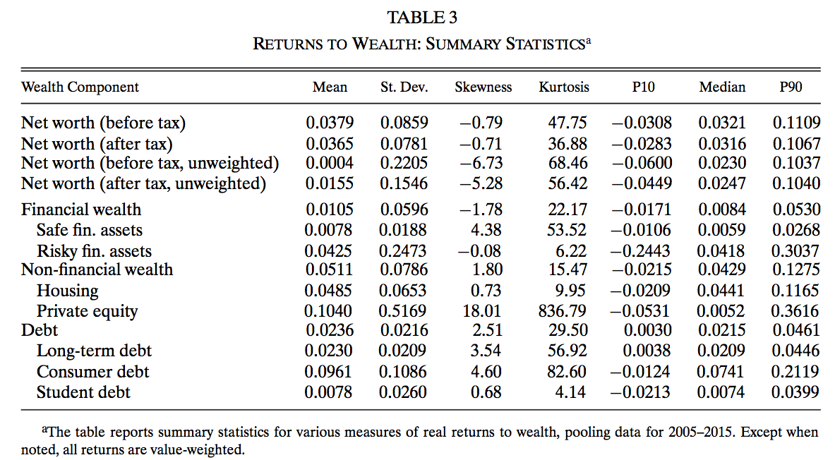
Source: Fagereng et al. (2020)
The point is therefore that returns matter. But returns will be a function of investment choices made by savers. In this set of lectures, we are interested in decision savers make regarding investment, how and when they invest, which are helpful to understand how these patterns arise.
One of the obvious place to start is to look at stock market participation. Why? Because the stock market has done historically much better in terms of returns than forms of investment which have less risk (such as government bonds). Using data from the U.S., the next figure shows historical returns on Equity (stocks) from the U.S. compared to 1 year Treasury Bills in the U.S. which is often used as a proxy for the safe rate of return. Since 1970, the average (nominal) return on equity is 11.8% compared to 5.5% for T-bills, a difference of 6.3% in return. Of course, investing on equity is more risky. The standard deviation of returns in equity is 17% compared to 3.7% with bonds.
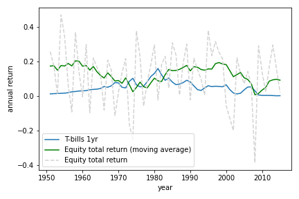
Source: U.S. Data from Jorda-Schularick-Taylor MacroHistory Database
To look yourself at the variation in returns over a long period and across countries, you can use this notebook.
![]()
For the data, you can download it here
Turns out lots of people do not invest in stocks. We can make use of data collected by the Retirement Savings Institute in 2018 to look into this. The next histogram shows among respondents age 35-55 in Quebec and Ontario the fraction of total savings in RRSP, TFSA and other taxable accounts which is invested in stocks. As one can see there is a significant group who do not put anything in stocks. There is also a sizeable group which puts everything in stocks. The distribution is relatively uniform within these bounds, with peaks at 20, 50 and 80%.
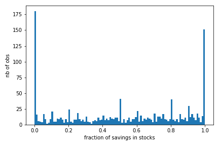
Source: RSI Survey on Retirement Savings Vehicles, Quebec and Ontario age 35-55. This extract contains data from 1305 respondents with positive savings in RRSP, TFSA or other taxable accounts.
Overall, as we show in the notebook below, the average share of savings invested in stocks is roughly 51.5%, 33.6% invest more than 75% in stocks, 13.3% do not put anything in stocks. The more educated, higher income, those with higher financial literacy put more in stocks. This may matter for understanding wealth inequality. As we show below the relationship between the share invested in stocks and both income and savings is particularly strong.
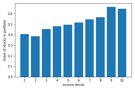
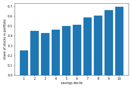
Source: RSI Survey on Retirement Savings Vehicles, Quebec and Ontario age 35-55. This extract contains data from 1305 respondents with positive savings in RRSP, TFSA or other taxable accounts.
You can investigate these differences using this notebook,
![]()
You can download the data here
It is worth asking why only half of savings, and for some even less, is invested in stocks given much higher returns. Obviously, risk aversion could play a role, but how much? This will be one of the topics below.
Turns out that when we look even within those who invest in stocks, there is substantial variation in returns as well as in risk in the portfolio held by investors. Lots of people are under diversified. The next figure from Campbell, Sodoni and Campbell (2007) shows just how under-diversified some investors are. Some obtain the same expected return but have portfolios with much larger standard deviation, which is, of course, not optimal if someone is risk averse. Seen in the other direction, some for the same amount of risk could increase their expected return by diversifying better. Diversification is a poorly understood concept. Even in our sample of investors, 14% of respondents judge a single company stock as risky as a mutual fund.
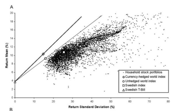
Source: Calvet, Sodoni and Campbell (2007).
This lack of diversification has welfare consequences. Another apparent puzzle is that despite large diversification benefits from buying international stocks within a portfolio, investors are biased towards domestic stocks, what is often called the home bias puzzle French and Poterba (1991). Here is what portfolios look like in three countries:
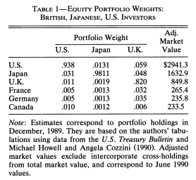
Source: French and Poterba (1991).
A more subtle puzzle is that when asked in the lab to allocate across different risky assets, some investors use simple heuristics, in particular one which leads them potentially to over-diversify by simply allocating an equal share of the endowment to different stocks.
In situations where taxes affect the rate of return on savings, some investors are better than others at taking into account tax considerations. This is the case for example in Canada with RRSP and TFSAs having different tax considerations and some investors suffer from important losses from not investing in the right tax-preferred saving vehicle (see Boyer, d’Astous and Michaud (forthcoming)).
If one invests in the wrong vehicle given marginal tax rates when contributing and withdrawing, mistakes can be substantial as the following figure shows. Hence, taxes matter.
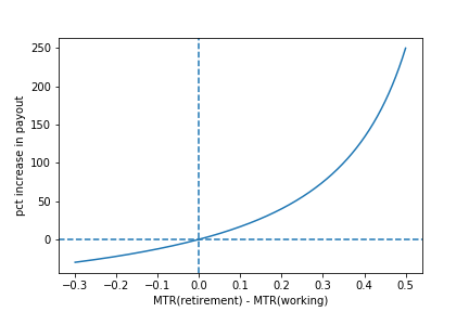
Source: Boyer et al. (forthcoming). The figure shows for an investor with a 30 year horizon the difference in payout (net after-tax withdrawal) for a 1000$ investment in a TFSA relative to an RRSP as a function of the difference in marginal tax rates. When the marginal tax rate difference is positive, the investor makes a better choice by using TFSA and the increase in the payout can be substantial. When the marginal tax rate difference is negative, the RRSP is a better choice.
A last set interesting facts as to do with how and when people trade. In particular, investors tend to trade often, suffering return losses, both because of trading fees and poor timing. This is the case in particular for males as shown in Barber and Odean (2001). The next table shows that men, in particular single men trade more often and obtain lower returns, relative to benchmark than women. Men are known to be overconfident and the authors argue that this is one the mechanism that leads to lower return for males.
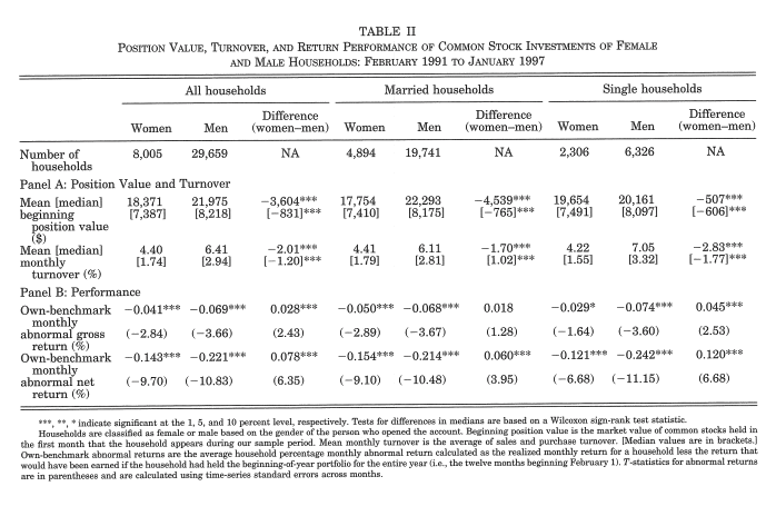
Source: Barber and Odean (2001).
The timing of their trading is also sometimes puzzling. Some investors sell stocks that have gained in value and hold on to stocks which have lost in value. Shefrin and Statman (1985) coin this the disposition effect.
Others participate in bubbles, thinking that the price can only go higher. Shiller (2000) is perhaps the most popular reference for this type of behavior which he calls irrational exuberance. The bottom line is that timing can also hurt returns in the long-run of when people buy and sell.
Theory
Consider an investor who has wealth \(w_0\) which he plans to allocate between risky assets and safe assets. Denote by \(\alpha\) wealth which would be invested in stocks. The return on the risky asset, \(\tilde{r}\) has expected return \(\mu_r\) with standard deviation \(\sigma_r\). The safe asset return is \(r_s\). Assuming expected utility, the problem is therefore :
where \(w = w_0 (1+r_s)\). The first order condition from this problem is
Assume utility has the form, \(u(w) = \frac{w^{1-\gamma}}{1-\gamma}\) where \(\gamma = R(w) = -\frac{u''(w)}{u'(w)}w\) is the coefficient of relative risk aversion and performing a first-order expansion of \(u'(w+\alpha(\tilde{r}-r_s))\) around \(w\), we obtain
The share is constant and does not depend on wealth. The share invested in the risky asset is inversely related to relative risk aversion \(\gamma\) and proportional to the risk premium (standardized using the variance of returns). This formula is simple to bring to data. From the historical data above, we had that \(\mu_r \approx 0.098\), \(r_s \approx 0.035\) and \(\sigma_r \approx = 0.17\). For a value of the share of wealth invested in the risky asset of approximately 50% as in the RSI data, one would need \(\gamma\) to be 4.4. In terms of the cross-section, this simple theory is problematic since those who do not invest in stocks would need infinite risk aversion. Furthermore, a value of 4.4 on average might be out of line compared to actual risk aversion if we measure it.
We have also seen that the share invested in stocks increases with savings, which violates the prediction of the simple unless risk aversion declines with savings in the data (those who are most risk averse accumulate more savings). This is a point forcelly made by Chiappori and Paiella (2011) who argue that it difficult to test whether risk aversion decreases with wealth using cross-sectional revealed preferences data since the observed relationship can be explained by both declining risk aversion as a function of wealth as well as a joint distribution of wealth and preferences. When using changes in wealth and the share invested in stocks, they cannot reject the null that the share invested in stock does not respond to changes in wealth.
Risk Aversion
How do we know if a value of 4.4 for \(\gamma\) is a reasonable value? Turns out there is a large literature trying to elicit values of risk aversion using experimental methods. One of the most famous study was conducted by Holt and Laury (2002) using Multiple price lists. Below is a Table showing the lotteries agents are presented.
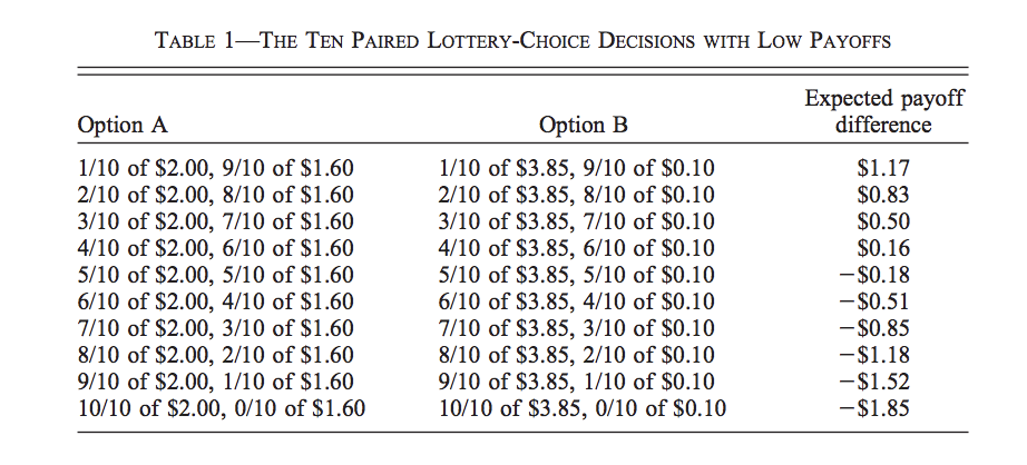
Source: Holt and Laury (2002)
Subjects will switch from lottery A to B as one progresses trough the table. The reason is that the expected gain difference between B and A grows as we proceed downward. At some point, subjects prefer the more risky lottery because they are compensated with a higher expected gain. In the last choice, one gets with probability one a higher payoff with B than A. In that paper, the authors assess the effect of paying subjects rather than presenting hypothetical lotteries. They also assess the effect of the scale of the gambles to see whether high stakes changes inferences. The next Table shows the results across the different experimental arms:
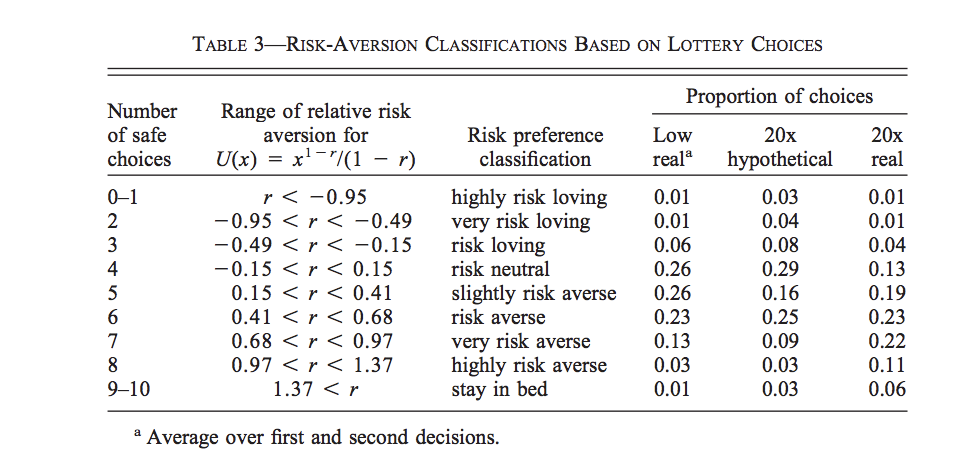
Source: Holt and Laury (2002)
In terms of hypothetical vs. real incentives, they show that there is a higher prevalence of risk loving subjects when using hypothetical lotteries. There is also more risk aversion when the real incentives are larger.
Values from Holt and Laury appear lower than the 4.4 value for \(\gamma\) needed to match the observed share invested in stocks. Boyer, d’Astous and Michaud (forthcoming) perform a preference elicitation exercise as in Holt and Laury with small real payoffs. The RSI dataset we used above to compute facts contains an estimate of relative risk aversion from this proceduce for each respondent. The average estimate of \(\gamma\) is 0.6. At this level of risk aversion, the predicted share is well above one and suggest that respondents should even be willing to borrow to invest with this risk premium on stocks. Hence, the expected utility model with CRRA preferences could not explain the facts we obtained from the data.
The equity premium puzzle follows from the fact that given a reasonable level of risk aversion, we should observe more much investment in risky assets. The puzzle was first discussed in Mehra and Prescott (1985). It has lead to a very large literature which we will not have space to cover. But we will look at two important behavioral explanations for this puzzle.
Finally, another interesting puzzle is that the fact that the share of stocks increases sharply with total savings does not appear to be due to decreasing risk aversion, or at least that this can explain very little of what we find in the survey. The next figure shows the average estimate of risk aversion by savings quintile. While there is some evidence of a decline, this decline is relately small and estimates are relatively flat starting in the 4th decile. Hence, the increase in the share of risky assets apparent in the data does not appear to be due to declining risk aversion.
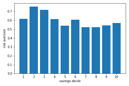
Source: RSI Survey on Retirement Savings Vehicles, Quebec and Ontario age 35-55. This extract contains data from 1305 respondents with positive savings in RRSP, TFSA or other taxable accounts.
Participation Costs
One way of explaining the behavior of those who do not invest anything in stocks is to introduce participation costs. These can be real (cost of opening a trading account, etc) or psychological, perhaps due to present-bias. Vissing-Jorgensen (2002) explores this idea and shows small participation costs can explain non-participation.
We can adapt our framework to seek the participation costs that would act as a lower bound that rationalizes the decision of our respondents. A respondent is indifferent between participating in stocks and not participating provided
where \(\tau_i\) is a participation cost. Conditional on participating, the optimal share is \(\alpha_i = w_i\) given what the risk aversion parameters we observe. Hence, the idea is to solve for \(\tau_i\), the participation cost that make this an equality for those who do not invest in stocks. One way to do this is to use a normal distributions for returns. The notebook below computes estimates of participation costs. Only a quarter of non-participants have costs lower than 150$, half lower than 755$. Hence, more than half require participation costs larger than 1000$ to rationalize their choices. Given how easy it is these days to buy an ETF fund using internet platforms for free, these participation costs remain a puzzle for this group.
Source: RSI Survey on Retirement Savings Vehicles, Quebec and Ontario age 35-55. This extract contains data from 1305 respondents with positive savings in RRSP, TFSA or other taxable accounts. Here only those with no stocks are included.
An important problem with this explanation is that participation costs cannot explain sub-optimal allocation to risky assets conditional on participating. Overall, while appealing, participation costs are a bit of a black box explanation for nonparticipation and not a good explanation for weights observed in the data.
Ambiguity Aversion
Turns out few of us know the distribution of returns and there is uncertainty about that distribution, in particular prospectively. The Ellsberg paradox shows that subjects dislike ambiguity, or the fact that probability distributions over states of the world are uncertain. When this happens, an action that involves an increase in ambiguity about the distribution of wealth will be of low value to that investor.
Here is how the Ellsberg paradox was shown. An urn consists 90 balls. 30 are red. The other 60 are either black or white. The proportion of white and black balls is not know. We ask you to make a choice between these lotteries:
Lotteries |
red |
black |
white |
\(L_1\) |
50 |
0 |
0 |
\(L_2\) |
0 |
50 |
0 |
Do the same in this context.
Lotteries |
red |
black |
white |
\(L_3\) |
50 |
0 |
50 |
\(L_4\) |
0 |
50 |
50 |
In the lab, lots will prefer L1 to L2 and then L4 to L3. But this is a violation of expected utility for any prior someone might have about the proportion of white and black balls (you can verify this easily). Both L1 and L4 have no ambiguity regarding payoffs while both L2 and L3 do. Hence, subjects exhibit ambiguity aversion.
One way to account for ambiguity aversion is to consider so-called multiple-prior models (Gilboa and Schmeider, 1989). In such models, agents are not sure what the distribution of risk is. For each state \(s\) the probability could take \(M\) possible values, \(P^m = {p_s^m}_{m=1,...,M}\). They attach a probability \(q_m\) that each distribution is the correct one. Under expected utility, this uncertainty does not matter because this is nothing else than a compound lottery and expected utility is linear in the probabilities. Hence, this just leads to a different weighting of the same final utilities in each state of the world. Hence, choices should still respect axioms of expected utility. An extreme form of ambiguity aversion preferences takes the form,
These are called maximin preferences. The investor considers the worst possible distribution in terms of expected utility. One can easily show that these can explain the pattern L1 preferred to L2 and L4 to L3 above. A smooth version of ambiguity aversion was proposed by Kilbanoff, Marinacci and Mukerji (KMM) (2005). If an investor has such preferences, the end result is that the investor is less likely to participate in the stock market if his priors are diffuse (the worst distribution is pretty bad in terms of investment results). She will also invest less in stocks.
But how to measure ambiguity aversion? Dimmock et al. (2016) propose a matching probability strategy. They provide subjects with a choice between,
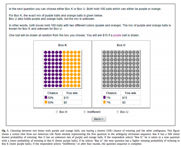
Source:Dimmock et al. (2016)
If the subject picks K in the first round, they lower the probability of winning from 50%. If the subject picks U in the first round, they increase this probability. They iterate until they find the probability that makes them indifferent. If the matching probability remains 50%, they are ambiguity neutral. If it is lower than 50%, the subject is ambiguity averse. The degree is ambiguity aversion is defined as 50% - q where q is the matching probability.
Source:Dimmock et al. (2016)
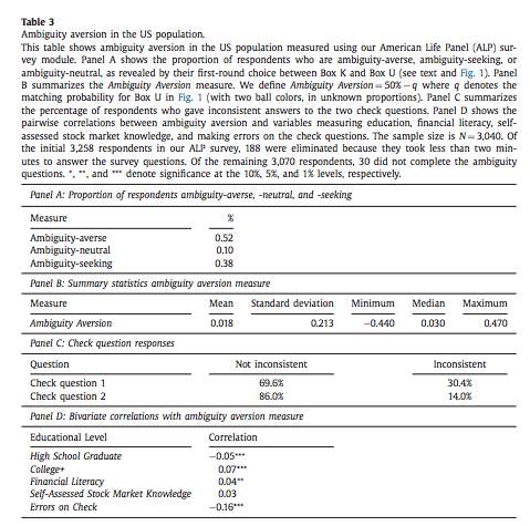
They tend regress stock market participation on their measure of ambiguity aversion and other controls. The next table shows the results. They find that ambiguity aversion reduces stock market participation.
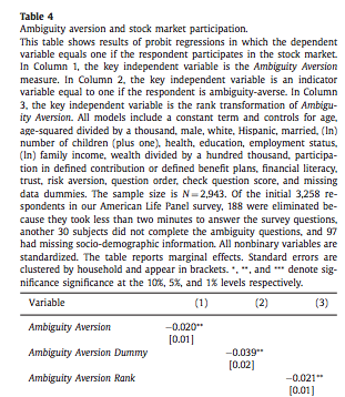
Source:Dimmock et al. (2016)
This theory shows promise to explain the puzzle. Many unexplored avenues for research exist in this stream. For example, one could elicit multiple priors from respondents. Another interesting avenue would be to relate ambiguity aversion to financial literacy. Perhaps one of the function of financial literacy is to reduce ambiguity.
Myopic Loss Aversion
Benartzi and Thaler (1995) provide a very interesting explanation to solve the equity premium puzzle. They combine loss aversion from prospect theory proposed by Kahneman and Tversky (1979) with mental accounting, as proposed by Thaler (1985). The first observation is that subjects in experiments tend to value gains and losses differently relative to a reference point. This is called loss aversion and is a key ingredient of prospect theory. A common utility function used is given by
where \(w\) is now wealth relative to the reference point, \(w_0(1+r_s)\). KT estimate \(\gamma\) to be roughly 0.88, while \(\lambda\) is close to 2.25. Hence, subjects tend to weight losses twice as large as gains. This may lower their demand for risky assets. This leads to a utility function of this sort.
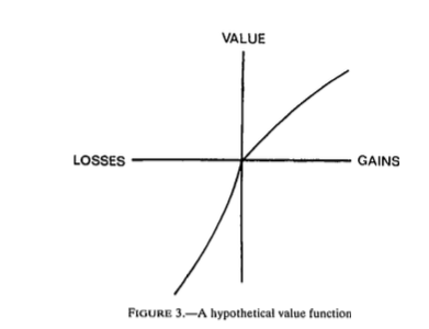
Source: Kahneman and Tversky (1979)
This tendency to weight losses more heavily than gains can be traced to particular regions of the brain. Tom et al. (2007) perform a loss aversion experiment by presenting subject lotteries while the brain is being scanned. They vary the gains and losses presented and record both choices as well as brain activity. Results look like this:
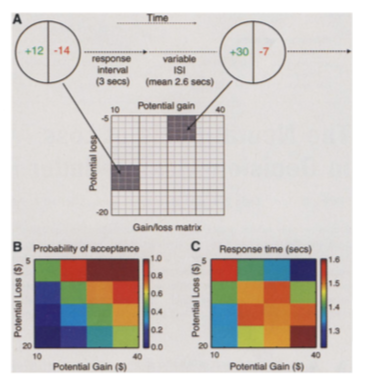
Source:Tom et al. (2007)
From these choices, they also estimate that the relative sensitivity of choice to losses was twice as large as for gains, consistent with evidence from KT. When they look at regions of the brain that are responsible for the sensitivity to gains and losses, they find, perhaps contrary to what some might expect that it is roughly the same regions of the brain which react. Hence, loss aversion is not the result of emotions such as fear (discomfort or vigilance).
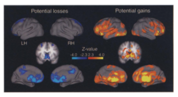
Source:Tom et al. (2007)
They estimate a similar relative sensitivity using neurological data (close to 2) which suggest that loss aversion emerges from a stronger rational or calculated sensitivity to losses than to gains.
Provided loss aversion is relatively strong, it could therefore explain low stock ownership.
But Benartzi and Thaler also raise an important issue in that one also needs individuals to be myopic in order for loss aversion to really bite. With loss aversion, the frequency at which utility is realized matters. The intuition is that if one only experiences utility 10 years from now relative to today’s wealth, then the distribution of gains and losses is different. If on the other hand, one experiences utility every month (checks on the market value of his savings), then he is likely to experience the loss domain more frequently. This breaks the invariance to the horizon which is present in long-term investing. When investors face iid returns, the sum of the returns over \(n\) periods is \(n\) times the variance of the one period returns. Hence, it is not true that the horizon lowers risk, something which Samuelson calls the time diversification fallacy.
Investors are likely to seek longer horizons, because they want to integrate losses and gains before experiencing utility, a mental accounting exercise first discussed by Thaler (1985). Waiting a long time means suffering from a huge loss only once. But that may be difficult to do with investing, when it is so easy to consult the market value of one’s portfolio. Therefore they may invest less in stocks than they would normally do. Benartzi and Thaler (1995) propose myopic loss aversion, the combination of loss aversion and short evaluation horizons as an explanation for the equity premium puzzle.
They simulate returns and evaluated utility at different horizons using loss aversion. The actual prospective utility function they use also take into account probability weighting and rank ordering which is also present in prospect theory (KT, 1979). The figure below shows that at evaluation frequency of less than 12 months, bonds dominate stocks while the opposite occurs when evaluation is infrequent. They also show that a mix of 50% stocks and 50% bonds appears to maximize roughly utility when prospective utility (with loss aversion) is used (at frequency of 12 months).
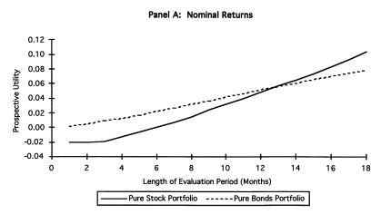
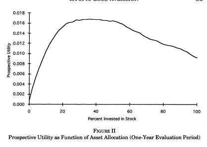
Source: Benartzi and Thaler (1995).
Diversification
So far, we have investigated the decision to purchase risky assets. The expected return on the risky asset did not depend on investment choices. Turns out investment choices can impact the expected return \(\mu_r\) as well as the standard deviation of the portfolio \(\sigma_r\). While it is obvious why the expected return matters, it is less obvious why the standard deviation does and how one can reduce it. In fact, risk-averse investors collect benefits from diversification, which is akin to the saying that one should not put all his eggs in the same basked. To understand diversification, consider the same framework as above but with two assets with returns \(\tilde{r}_1\) and \(\tilde{r}_2\) with identical expected returns \(mu_r\) and standard deviation \(\sigma_r\). The consumer aims to decide how much to invest in the first asset,
The first order condition is
which yields the solution \(\alpha^* = \frac{w}{2}\). While the expected return of the portfolio is \(\mu_r\), the standard deviation is now \(\frac{\sigma_r}{2}\). Since the returns are iid, the variance of the portfolio is reduced by diversification. When expected returns and standard deviations differ across assets, diversification benefits still occur but the optimal solution will be slightly more complicated. Returns may also be correlated.
One of the most celebrated models of portfolio choice is the mean-variance model which highlights the return - risk tradeoff. Depsite its simplicity it is still one of the workhorse models of portfolio theory.
Consider \(K\) risky assets and the return on each of these \(\tilde{r}_k\) and a safe asset with return \(r_s\). The expected return of each is \(\mu_k\) while the covariance between two assets \((j,k)\) is \(\omega_{i,j}\). The covariance matrix is \(\Omega\). Wealth is therefore given by
The portfolio share for the safe asset is \(1-\sum_{k=1}^K \alpha_k\). Let us assume the agent picks these portfolio weights so that
where \(\mathbf{\alpha} = (\alpha_1,...,\alpha_K)\), \(A(w_0) = - \frac{u''(w_0)'}{u'(w_0)}\) is absolute risk aversion and \(V_r\tilde{w}\) is the variance of wealth. For CRRA utility, \(A(w_0) = \frac{\gamma}{w_0}\)
We have that
and
Hence, the first order conditions for this problem yield:
Wealth \(w_0\) cancels out. It is useful to rewrite in matrix form,
which can be solved to obtain,
and the share in the safe asset is \(1-\sum_{k=1}^K \alpha^*_k\). Two important observations: 1) risk aversion impacts the fraction of risky assets in the portfolio but not the allocation of wealth across risky assets. The same factor \(\frac{1}{\gamma}\) appears for each risky asset. 2) The optimal allocation of risky asset depends on the returns and covariance matrix of returns only. Take the case where returns are independent. Then the optimal share of risky asset \(k\) is \(\frac{1}{\gamma}\frac{\mu_k - r_s}{\omega_{k,k}}\). The optimal share depends on the risk premium, \(mu_k - r_s\) and negatively on the variance of the risky asset. Overall the composition of the portfolio does not depend on preference. There is an optimal mix, or mutual fund that agents can pick and only the decision of how much to allocate to this fund depends on preferences. This result is often referred to as the two-fund separation theorem.
The following notebook computes optimal weights for a given set of assets, which includes a safe asset. It considers the SP TSX composite index and the MSCI world index. Hence, these are two diversified indices. When considered jointly, the investor is willing to invest most of his wealth in such a portfolio, achieves higher returns and higher utility. When we restrict only to the SP TSX, the investor has lower utility and in this case lower returns. Hence, even though the two indices are quite correlated (correlation at monthly level = 0.6), there are still benefits to diversification.
For the notebook, you can open it here
![]()
You can download the data here
The home equity bias states that investors appear to disproportionally prefer home stocks. Using the mean variance model, one can compute the expected return that would be needed to rationalize observed allocations. From the table below taken from French and Poterba (1991), we can see that we would need much higher home returns.
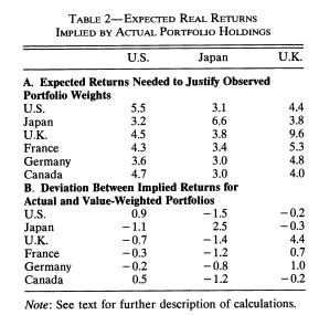
Source: French and Poterba (1991).
Explaining the lack of diversification in portfolios, in particular home bias, can be done in several ways. One is ambiguity aversion. Knowning the returns on certain costs better than others certainly tilts the portfolio towards those. Maybe investors know home stocks better than international ones. Another is simply that the computational cost is high and cognitive skills may be at play. Finally, financial literacy can also explain the lack of diversification. van Gaudecker (2014) shows that those with much higher financial literacy do better but that those with low financial literacy who trust their own abilities tend to do much worse. Decision aids which help with figuring out the effect of diversification may be particularly effective.
The opposite mistake is also common, i.e. over diversification. In particular, Benartzi and Thaler (2001) show that many use a simple heuristic, \(1/K\) where \(K\) is the number of choices in the plan. As a result, the fraction invested in stocks increases in plans where there are more options (more generally is a function of the menu). Again, decision aids could help investors avoid the use of such heuristics.
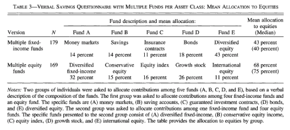
Source: Benartzi and Thaler (2001)
Other Issues
Investors have a hard time dealing with fees which are involved when investing in mutual funds. In one important study, Choi et al. (2010) show that more than 80% of subjects in an experiment fail to minimize fees when picking mutual funds. Financial literacy lowers fees paid. Fee disclosure is now common in many countries. But even when they are disclosed investors do not always minimize fees or know how to integrate this information into their decision making.
Clark et al. (2015) show that those with higher financial literacy obtained higher returns on the savings, and had less idiosyncratic risk in their investment choices suggesting they diversify better. This could suggest that interventions aiming to increase financial literacy may help with diversification.
Interventions
Financial advice
In principle, advisors could be a substitute for financial literacy and investment knowledge. They could help investors get better returns. In a world where advisors are benevolent and there is no asymmetric information, this could certainly be the case. The extent to which they will do so depends on the compensation structure of advisors, or incentives more generally.
A good survey of the literature on modeling and regulation is provided by Inderst and Ottaviani (2012). Studies on the value of financial advice and its effects are rare and only starting to emerge.
Hackethal et al. (2012) show that advised accounts at a large broker firm reach lower net returns and inferior risk-return tradeoffs compared to self-managed accounts. On the other hand, Bluethgen et al. (2007) find that advised clients are more diversified but pay higher fees. Hence, this remains an open question.
A famous study which demonstrates that conflict of interest likely decreases the efficiency of financial advice is Mullainathan et al. (2012). They use an audit study to show that often advisors reinforce biases of their clients in a way that is profitable to them. When there is asymmetric information, there is the potential for investors to not be able to distinguish between high and low quality advisors. They consider four scenarios: a return chasing scenario, a company stock scenario, a well-diversified scenario and finally a control group where the investor only has cash. These scenarios are randomized. Advisors are much more sympathetic to the return chasing scenarios (which increases their compensation from frequent trades), less sympathetic to the company stock (which minimizes transactions). Interestingly, they are unsupportive of the well-diversified efficient portfolio. Advice favoring stocks was more likely for higher income investors. But they advised against more equity exposure as the amount invested increased.
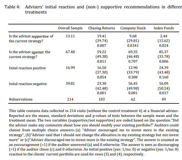
Source: Mullainathan et al. (2012)